Breaking Down My Master Thesis
Motivation Behind the Topic
A little over a decade ago, a new genre emerged from the depths of the Russian rap scene. As of now, it has no name (to my knowledge) and can take many forms, though it usually appears as rap. The genre’s distinctive feature is highly conceptual, linguistically experimental, neologism-heavy lyrics. Examples of artists include Ezhemesyachnye, Husky, makulatura, Krovostok and Pasha Technique. I think a name like “solyanka” can stick. Solyanka is a common dish, or rather, a culinary disaster of one, in post-Soviet countries, whose name became a phraseological unit meaning ‘a mix of everything’. In this context, solyanka is used as a metaphor for content-rich. One could argue solyanka the dish is as abstract in its contents as the music of the aforementioned bands.
Apple Music was not able to reliably distinguish between rap and solyanka, often creating poorly assembled playlists for me. Classifying solyanka versus not solyanka is a rather thrilling challenge, but too narrow for a master’s thesis. Instead, I decided to explore whether modeling lyrics — the defining feature of solyanka — could improve the performance of content-based music recommendation systems in general.
Why It Matters
Predicting which songs a user might like based on the listening histories of similar users generally yields a better result than using only content-based methods (audio, metadata, etc.). However, when songs have few or no streams — which is common for solyanka — content-based methods are the only viable option for recommendations. This makes it essential to find effective ways to represent song content in a computer-friendly manner.
To achieve this, I created multiple variables to model the complexity of song lyrics. Four of these variables significantly improved recommendation quality, including two which could be directly linked to solyanka: MTLD and lexical sophistication.
- MTLD (Measure of Textual Lexical Diversity) is calculated relatively simply and measures the proportion of unique words in a song. It is widely used in linguistic assessments and has applications in monitoring language impairments. Interestingly, MTLD also proved useful in predicting songs a person might enjoy.
- Lexical sophistication is the percentage of words not found in the 5,000 most commonly used words. I used the same method that Grammarly employs to calculate its sophistication index.
You can find the list of all variables in my paper.
Why It’s Difficult (or Nearly Impossible)
Solyanka, however, is not characterized just by lyrical complexity. It is a genre deeply rooted in the Russian culture and mindset, both of which are arguably impossible to model. In music recommendation literature, this phenomenon is called the Semantic Gap.
“The semantic gap is the discrepancy between what can be extracted from music (i.e., semantic or audio features), and high-level human perception of these features”.
One way to bridge the semantic gap is by modeling as many features as possible. In an ideal scenario, a data-omniscient supercomputer could fully capture the intricacies of solyanka, eliminating the gap altogether.
Feature Importance and Weighting (Not Included in the Paper)
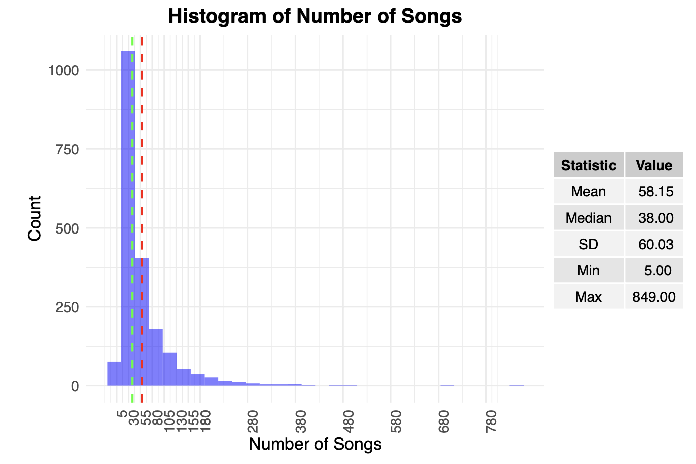
One major idea I had was to account for the varying importance of features for different users. While this is not groundbreaking, it becomes a challenging task when a user has only a few streamed songs. In my dataset, most users had under 38 unique streamed songs. With over 70 features and only 38 observations, calculating feature importance became a major challenge due to the curse of dimensionality and the risk of overfitting.
For song similarity calculations, I used weighted cosine similarity as implemented in scipy:
\[\theta = \dfrac{\sum_{i} w_i u_i v_i}{\sqrt{\sum_i}w_i u_i^2 \cdot \sqrt{\sum_i}w_i v_i^2}\]To determine weights for individual variables, I used a transformed version of their feature importances/coefficients, calculated through a classification task: predicting whether a user listened to a song more than the average number of times.
Finding the optimal weights for each variable posed another challenge. A naive approach like random search was infeasible: with just 10 variables and 10 possible values each, the search space ballooned to 10 billion combinations. Instead, I needed a more efficient approach based on available user data.
Below are the R implementations for linear SVM and XGBoost used to calculate user-specific feature weights:
calculate_user_weights <- function(user_song_profiles, user_utility_vector) {
  set.seed(7)
  data <- data.frame(cbind(user_song_profiles, user_utility_vector))
  colnames(data)[ncol(data)] <- "utility"
  data$utility <- ifelse(data$utility >= mean(data$utility), 1, 0)
  data$utility <- as.factor(data$utility)

  classifier = svm(formula = utility ~ .,
                   data = data,
                   type = 'C-classification',
                   kernel = 'linear',
                   class.weights = "inverse")

  weights_vector <- t(t(classifier$coefs) %*% classifier$SV)

  set.seed(NULL)
  return(normalize(weights_vector))
}
calculate_user_weights <- function(user_song_profiles, user_utility_vector) {
   set.seed(7)
   data <- data.frame(cbind(user_song_profiles, user_utility_vector))
   colnames(data)[ncol(data)] <- "utility"
   data$utility <- ifelse(data$utility >= mean(data$utility), 1, 0)
   data$utility <- as.factor(data$utility)
   class_freq <- table(data$utility)
   num_samples <- nrow(data)
   num_classes <- length(unique(data$utility))

   data$weight <- num_samples / (class_freq[as.character(data$utility)] * num_classes)
   data$weight <- ifelse(data$weight == max(data$weight), data$weight*10, data$weight)

   weights <- data$weight

   xgb <- caret::train(
     utility ~ .,
     data = data[, -ncol(data)],
     method = "xgbTree",
     weights = data$weight,
     trControl = trainControl(method = "cv", number = 5),  Using 5-fold cross-validation
     tuneGrid = expand.grid(
       nrounds = 1000,
       max_depth = 1,
       eta = 0.025,
       gamma = 0,
       colsample_bytree = 0.2,
       min_child_weight = 0,
       subsample = 0.7
     )
   )

   predictor <- Predictor$new(
     xgb,
     data = data[, -ncol(data)],
     predict.fun = function(object, newdata) {
       predict(object, newdata)
     }
   )

   imp <- FeatureImp$new(predictor, loss = "ce")

   weights_vector <- as.matrix(imp$results$importance)
   rownames(weights_vector) <- imp$results$feature

   return(weights_vector)
}
Results
Using SVM, the model showed significant overfitting, as shown in the MAP@500 scores:
| Dataset | MAP@500 |
|---|---|
| Weighted Test | 0.00251007 |
| Unweighted Test | 0.00236711 |
| Weighted Train | 0.04017487 |
| Unweighted Train | 0.03838689 |
While the weighted model performed worse on training data, it improved test set precision by 6%, suggesting potential benefits in real-world scenarios.
A large overfitting of the model can be observed in the results above with the large differences in MAP@500 between train and test. Moreover, while weighted model performed worse on train data, it managed to improve the precision by 6% on test data.